EDA file format considerations
1. Introduction
In this article we will focus on Electronic Design Automation (EDA) file formats, more specifically formats that are designed to describe a Printed Circuit Board (PCB).
There are many different ways a PCB file format can be made. The focus of this article is showing the most common aspects which are usually design decisions when creating a new format. We will enumerate a custom set of such aspects and demonstrate them by examples in existing file formats.
In chapter 1, a rationale is presented for the importance to consider these aspects. In chapter 2 the problem domain is partitioned into two, mostly independent levels. In chapter 3 and 4 these two levels are discussed in details. Finally, in chapter 5 hints are given for documenting the file format.
1.1. Design for others and for long term
It is possible that a new PCB file format is created by randomly making these choices. If then a complete, proper implementation is developed for one software which then has a final version and there is no further development, the actual choices matter very little.
However, in practice this rarely happens; instead:
- the format needs to be maintained for decades, with new features added, old features removed or changed as the software evolves
- other projects developing independent
- some implementations will choose to support only parts of the specification
- and some implementations will have bugs
If compatibility arcing between versions decade apart of the original software, and/or interoperability with other software through this file format is important, then those initial choices start to matter a lot. In fact, a few bad choices may be a source of constant struggle and limit the maintainer to make further suboptimal choices down the road as the format evolves. Thus it is very important to be conscious about the possible long term effects of those design decisions from an early stage of the file format design.
1.2. Consistency
One of the most important factor in keeping the format clean on long term is understanding the data the file format will need to express and choosing format details so that the same or similar kind of things are always expressed the same or similar way. Or in other words, the file format design is consistent. This requires early decisions to consider possible (or most probable) future directions of the file format.
But it also requires discipline: once a choice is made about how something is expressed, a decade later in for a similar feature the format should try to use the same (or similar) syntax. Even if by now, or for the new feature a different syntax could be more elegant.
A good example is how coordinate units are expressed in a KiCAD s-expression board file: the format is specified so that all coordinates are in mm, using floating point in decimal. tEDAx does the same. Another good example is pcb-rnd's lihata board where each coordinate string has a unit; this makes mixed-unit design easier to store without losing precision.
A bad example is PADS ASCII: for object rotation, degrees are used in floating point, to multiple decimal digits; for arc angles integer degrees are used with a fixed *10 multiplier. This is an incosistency, the same type of thing expressed differently, using different unit and numeric format when it is stored in different object fields.
1.3. Avoid assumptions
A good design is not a random collection of solutions tailored for very narrow, specific use cases, but a collection of general purpose tools that can be combined in arbitrary ways. Creative users can solve problems not foreseen by the designer by using unexpected combinations. The least the design assumes about how exactly the format will be used, especially what exact use cases will be stored, the more flexible it is and the more unforeseen problems it will be able to solve.
A good example is how footprints are modeled in pcb-rnd using subcircuits. A subcircuit is essentially a generic group object; the most important part of a subcircuit is the so called data subtree, which holds all drawing primitives. The exact same data subtree is used for the board, thus anything that can be drawn on a board can be drawn in a footprint too.
A bad example is gEDA/PCB's element for footprints. In this model there is a set of drawing primitives for a board and a disjunct set of drawing primitives for elements. Thus a footprint can have only a few different features and extending this would require introducing new drawing primitives which is expensive both in code and in file format. If this effort would eventually reach the state where anything could be drawn on a footprint that could be drawn on a board, that'd mean the whole code and file format is duplicated in two copies, one for the board, one for footprints.
1.4. Format scope
A board file normally consists of vector graphics and metadata, such as:
- components (parts that will be soldered onto the board)
- the netlist (logical connections between component pins)
- the layer stackup (Figure 1)
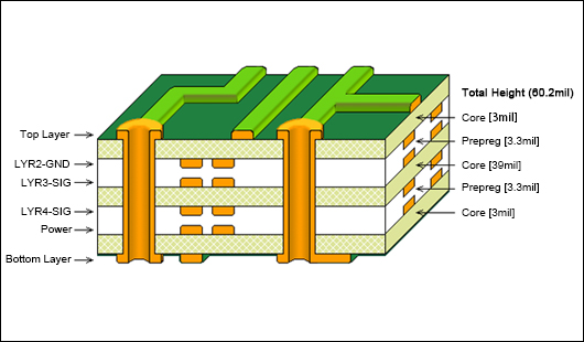
Figure 1: Layer stackup shown on a board cross section; golden: copper tracks and the via (the two "tube" constructs); core and prepreg are insulation layers; the thin green paint above the top layer and below the bottom layer are called the "solder mask" and is a solder resist lacquer which has cutouts to expose bare copper where soldering should take place.
The vector graphics consists typically of lines, arcs, polygons, holes and in vast majority of file formats text objects. An EDA-specific aspect is expressing footprints, which are the land pattern (e.g. holes and copper pads for the pins) of components that will be soldered on the board.
2. File format vs. data model
2.1. Different levels of representation
In this document, we make a clear distinction between file format and data model. The file format is the low level packaging of the high level data model. The file format determines how exactly a string is encoded, but the meaning of the string is defined by the data model.
For example SVG has XML as the low level file format. With that design decision SVG does not need to invent and specify its own way how to represent a tree structure in a text file, how to quote multi-line strings, etc. However, XML itself is a generic format, it does not know anything about graphics. Majority of what makes SVG so complex is not on the file format level, but on the data model level: how SVG defines drawing primitives like paths and how it handles special cases like self intersecting polygons.
For example consider the following SVG drawing and the corresponding render (Figure 2):
<?xml version="1.0"?>
<svg xmlns="http://www.w3.org/2000/svg" ... >

<g id="layer_3_top">
 <line x1="8.2550" y1="13.3350" x2="8.2550" y2="1.9050"
       stroke-width="0.2540" stroke="#8b2323" stroke-linecap="round"/>

 <path d="M 8.25500000 1.90500000 A 6.3500 6.3500 0 0 0 1.9050 8.2550"
       stroke-width="0.2540" stroke="#8b2323" stroke-linecap="round"
       fill="none"/>

 <circle cx="6.9850" cy="12.0650" r="1.0000" stroke-width="0.0000"
         fill="#707070" stroke="none"/>

 <circle cx="6.9850" cy="12.0650" r="0.4001" stroke-width="0.0000"
         fill="#ffffff" stroke="none"/>
</g>

<g id="layer_9_outline">
 <rect x="0.0000" y="0.0000" width="10.1600" height="15.2400"
       stroke-width="0.2540" stroke="#00868b" stroke-linecap="round"
       fill="none"/>
</g>
</svg>

Figure 2: example SVG rendered.
The low level is called XML; in the above example it is the way how tags ("commands") are given in <> or how their attributes ("arguments") are specified within the <> element. The high level is how we define rect or path should behave, how these instructions are translated into pixels.
In an ideal world the data model is designed first and the file format is chosen later. This is the essence of any CAD program:
- this determines what data the CAD operates on
- it is the window from the CAD program and the reality it tries to model
- as a result determines the features, limitations and quirks of the modeling
- it also can be regarded as the mapping between UI features and the file format
Once the data model is designed, a suitable file format should be chosen: a format that can accurately represent the data model, with all considerations of chapter 1.
2.2. Example: eagle binary -> XML
There are usually multiple file formats that can represent the same data model. A good example is eagle: around version 6 the file format changed from a custom binary format to XML. We support both file formats in pcb-rnd. It was relatively easy because the data model did not change, only the low level format: we started with eagle XML support. With that we learned the data model. Once it reached mature state we started to figure how the binary file is structured, looking for the same data model in it. Our implementation is clearly separated into a high level data model parser (Figure 3), that operates on an abstract tree. The abstract tree is extracted from the file format using libxml2 for XML for new files and custom code for the old, binary files.

Figure 3: how Eagle binary and xml files (top) are processed and translated by different code layers until data is converted to pcb-rnd data model; concepts equivalent on the binary and xml path are in the same row on the drawing.
2.3. Format is cheap, model is expensive
It is important to note that the a properly chosen file format does not play a role in the capabilities of a CAD software. The wrong file format can obviously limit what the data model can express, but assuming the file format is chosen from the set that is suitable for presenting every detail of the data model, the actual choice really does not matter much.
This is often overlooked by users pressing for a specific file format. For example in case of gEDA/PCB, file format was a recurring topic on the mailing list between 2010 and 2020: users bumped into various limitations of the software which they often viewed through the saved board file. Some users had the impression that the limitation is imposed by the file format, because they knew the given file format and saw that it did not have a way to express the feature they longed for. Back then some users proposed to switch to XML or json, markdown or even SQL.
However such a switch in the file format would not fix the problems, because the missing features are also missing from the data model. While gEDA/PCB's file format is not that well designed, it could be extended to represent majority of the missing features, and that would be the smaller part of the work. The larger part is extending the data model and upgrade the code base for it.

Figure 4: an EDA software stack: features display and manipulate the data model, file formats are just low level representations of the data model.
pcb-rnd started as a fork of gEDA/PCB. In 2017 we started to redesign the data model. Since we decided to keep pcb-rnd operational and compatible during the transition, the project took one and a half years (during other, normal development). We used an already existing low level file format, lihata. Evidence shows that switching the file format from a custom, positional text format to lihata was a very small part of the time spent (about 6% at that specific stage) while bulk of the time was spent on the pcb-rnd core code upgrades for the new data model.
2.4. Native vs. exchange formats
There are some file formats and data models that are intended to be the native of a specific software. The native model is the actual core code of the given software: this is how the software represents the world it is aware of. The native format is normally designed to be an 1:1 mapping of the native data model.
A file format designed for data exchange between different software normally also needs to have its own data model that is independent of the native model.
The main difference between native and exchange is some core design decisions. Whenever there are tradeoffs between "easy to understand, easy to implement, concept likely to exists in any other software as well" and "specific feature needs to be supported, whatever it takes in the model or the file format", the decision should consider whether the design is for native or exchange.
3. Low level: file format
3.1. Perceived portability
For a native data model portability among different software is not a requirement: each software package has its own native model. The associated native file format is usually not designed to be portable either: it is not practical as an exchange format as it is tightly coupled with the native data model more geared for implementing specific features than for simplicity or generalism.
On the other hand an exchange file format needs to be portable between software packages and it is also a reasonable requirement that it shall be easy to implement.
The latter is very often attempted by using an existing file format with well established libraries instead of inventing a custom format. Some file formats, like xml, json files are very easy to read and write with any programming language, because there are libraries already implemented. However, this is only perceived portability if the file format is not very easy to reimplement. There can be many reasons why libraries can not be used:
- licensing issues
- library doesn't yet exist for the programming language chosen for the project
- the library is huge and can not be easily compiled on the target platform
- the 3rd party supplier of the library abandons the project; the library is too large and nobody stands up to maintain it
Thus relying on 3rd party libs for the format can easily become perceived portability.
An alternative is simplicity, which can mean using custom file formats. There are a few basic file format types that are really easy to load with any reasonable programming language or system that existed in the past 30 years:
- plain text, positional
- plain text, named fields
- plain text, s-expression
If it is done right, and the format is kept as simple as possible and is well specified, implementing custom code for the format can be cheaper than maintaining the build system, dependency and APIs to a format library. A good example on this is tEDAx, which has very small parser reference implementations:
| language | size in sloc |
|---|---|
| C | 66 |
| AWK | 29 |
| python3 | 64 |
| welltype | 72 (estimated) |
3.2. Text vs. binary
Whether the format should be text or binary greatly depends on the nature of the data model.
For example an SVG is very easy to store in text because it mostly consists of drawing primitives and properties that can be represented by keywords and a few coordinates and other numeric data that are also easy to encode in text. With some trickery, it is possible to reasonably extract data from SVG with text processing tools. It is simple to write code that emits SVG in any language. Advanced users often use a text editor to modify SVG files.
Meanwhile bitmap formats, like png or jpeg have bulk pixel data. Even if a format can represent them in plain text, such as some levels of the pnm format, it's rarely useful with text processing tools. It is also rare that someone would use a text editor to manipulate a largish bitmap. Thus binary format for this kind of data is more justified. Further examples are raw digital sound and video streams.
If file size is concern, a well designed text format can usually be efficiently compressed.
Most data are not cleanly text-only or cleanly binary-only by nature, but they are somewhere in between. Since it is possible to store binary data in a text file with proper encoding (e.g. base64) and it is trivial to store text data in a binary file, the question really is whether the nature of the data model is closer to text or closer to binary.
EDA data models are closer to SVG than to png, and thus are closer to text than binary. Most EDA related file formats are therefor text based.
3.3. Flat vs. tree
This clearly depends on the data model, which will be discussed in chapter 4. Most EDA related data models are trees, thus they are easier to translate to a file format that natively support representing trees (for example XML or json or lihata). If the file format chosen does not support trees, there are ways to emulate them; this will be discussed later in this chapter.
3.4. Text file format considerations
3.4.1. Field encoding
Independently of the file being flat or a tree, there will be objects and objects will have multiple properties or fields. There are two commonly used method for storing fields of an object: positional and named fields.
3.4.1.1. Positional files
In a positional system there is an ordered list of fields, very often a a space separated list of words in a line of text, and the meaning of the given field (word) is specified by it's position within the line. For example this is how an arc object looks like in tEDAx:
arc primary silk - 3.81 -1.27 1.27 0.0 180.0 0.2540 0.0
where the first word specifies it will be an arc, the second and third word specify the layer, the 4th word is the terminal ID, then come center point coordinates, radius, start and span angles (0 and 180), stroke width and clearance.
A similar, but less clear positional format is the gEDA/PCB board file format:
Arc[342519 204724 31496 31496 3000 5000 0 -90 "clearline"]
Layer information is given elsewhere, coordinates are in a different unit, order of fields differ too, but the generic idea is the same. It's less clean because it uses [ and ] as special field separator.
A positional file format is easy to read only if there is a formal limit on the line length: most programming languages offer a standard library call to read a line of text from a file and then it's usually easy to split it up. Without a line length limit in specification, a more complicated tokenizer needs to be used.
Some positional formats have optional fields: after a specified amount of fixed fields, typically at the end of the line, there may come a fixed or varying amount of fields (vararg) that can be omitted.
Positional file formats are very dangerous on the long term: as long as
- there are only fixed fields;
- and any new version only extend the number of fields but do not remove or change the meaning of existing fields
compatibility can be maintained. However, as soon as optional or vararg fields are added to a line, new fixed fields can't be added without earlier versions of code mistaking them for optional/vararg fields.
For example Qucs uses an xml-lookalike custom format witout attribute names, so that the attributes for a tag is really an ordered list. This is a non-line based, positional format. For the <R> tag within the <Components> subtree
	<Qucs Schematic 0.0.17>
	  <Components>
	    <R R1 1 340 130 -26 15 0 0    "1 Ohm" 1 "26.85" 0 "european" 0>
	 </Components>
A special case of positional formats is when fields are not separated by field separator sequences but start at specific column (character offset) within the line. This format was popular in the age of punch cards and punch tapes. Probably the most famous such format that has a descendant that is still in use is the original Fortran format. An EDA example is the IPC-D-356 electric tester format:
C  IPC-D-356 Netlist generated by gEDA pcb-rnd 1.2.6
C
C  File created on 2018-04-13 06:44:02 UTC
C
P  JOB   7805.pcb
P  CODE  00
P  UNITS CUST 0
P  DIM   N
P  VER   IPC-D-356
P  IMAGE PRIMARY
C
327unnamed_net2     C3    -1          A02X+010354Y+004000X0511Y0590R000 S2
317unnamed_net2     CONN2 -1    D0393PA00X+002500Y+004000X0800Y0800R000 S0
317unnamed_net2     U1    -3    D0600PA00X+010000Y+002750X0900Y0000R000 S0
327GND              C3    -2          A02X+009645Y+004000X0511Y0590R000 S2
327GND              C2    -2          A02X+008354Y+004000X0511Y0590R000 S2
Lines starting with C and P are comments and headers. Data lines start with a 3 digit integer keyword. Note how there is no space between the keyword and the following field, which is a netname.
3.4.1.2. Named fields
In the named fields setup each field is a key-value pair. The meaning of the field is specified by the key with is explicitly spelled out for each value. Most often the order of fields does not matter.
For example an arc in the lihata board format:
ha:arc.695 {
  x=2.975mm; y=47.625mm; width=25.0mil; height=25.0mil;
  astart=270; adelta=-180; thickness=10.0mil; clearance=0.0;
}
Such file format is more verbose and encodes the same amount of data in much more bytes, making the files bigger on disk. However, they are much easier to maintain long term: adding or removing named fields, using variable number of fields will not break compatibility as long as unique field names are specified.
An interesting variant is BXL's semi-s-expression syntax:
Line (Layer TOP_SILKSCREEN) (Origin 900, 400) (EndPoint 900, 410) (Width 1)
Unlike a real s-expression, the file is line based and lines normally start with a keyword. Arguments are then grouped in s-expression-like () subtrees, where the first word is the field name. Note how this allows multi-data fields, like x,y coordinates.
Another interesting and rare variant is the single-field-per-line, as demonstrated by protel netlist version 2.0:
[
DESIGNATOR
X1
FOOTPRINT
TO220
PARTTYPE
Macro
DESCRIPTION
3-Terminal Adjustable Regulator
PART FIELD 1

LIBRARYFIELD1 1

]
Each key-value pair is given in two lines, first the key, then the value. In this syntax both the field and the record separator is the newline sequence.
3.4.2. Strings: escaping and quoting
A crucial detail to specify in a text format is how strings are escaped. Text formats have control sequences used for field or record separators or open/close. These sequences embedded may occur in data strings as well where the shall not be confused with file format level control.
There are mainly two strategies for this:
- "rest of the line" vararg"
- escaping specific characters
- quoting strings with the same character
- quoting strings with open/close
The cheapest, but least portable (in time) way available in a line based text file is having only one string field per line, as the last field and specify it as "anything from the 4th field till the end of the line is the string". However, this method has severe limitations: once such a field is added, the file format on that line can not be extended in a compatible way, and newlines still can not be encoded in the string without breaking the format. For example in a gEDA/gschem schematics file, a device attribute line looks like this:
device=ceramic capacitor
This file is not strictly positional, the above line is a key=value, where value does not need escaping because anything after the '=' sign is considered to be the value. However, '=' can not be in the key (version 1.8.2. GUI allows this tho and becomes inconsistent after saving and reloading the file!), plus newlines in value are protected by a different mechanism.
In escaping, control characters or sequences are escaped by prefixing them with a special character, usually the backslash. This yields a special case: if the string needs to contain a literal backslash, that needs to be escaped too, else it's taken as a backslash escape for the following character. If there is no string quoting, this is a simple, flat method. For example tEDAx uses whitespace for field separator so spaces in text string fields need to be protected with backslash:
device C1 ceramic\ capacitor
In the above tEDAx netlist example the line contains the device keyword then two fields: refdes and description. The description field contains a space, which is escaped with a backslash, thus the line contains only 3 fields, the 3rd field being ceramic capacitor.
The alternative is to quote strings. A quoted string usually starts with a single or double quote and ends with the same quote character. Within a quoted srting characters used in the file format syntax (e.g. field separators) don't need to be escaped separately as the quoting means: "take all character until the end of the quote as literal, do not interpret them". For example the above line in ACCEL_ASCII netlist format would be:
compRef "ceramic capacitor"
This line contains only two words (the refdes is specified elsewhere): a keyword and the text value. The text value is quoted using the double quote character. This allows any other character than the closing double quote to appear in the string without escaping. However, escaping is still needed if the string contains the quote character. Usually backslash is chosen for the escape character, and literal backslash then needs to be escaped too, so at the end such quoted strings usually have \" and \\ as special sequences.
Finally, a special case if quoting is when different opening and closing character is chosen. This has the adventage that when multiple strings are quoted in a line, fields are easier to see. For example consider the following two lines of hypothetical line based text formats, first using double quotes, the second using curly braces for quoting strings:
print "hello world " "this is a" " string split" " in fields with " spaces
print {hello world } {this is a} { string split} { in fields with } spaces
Advantages: different opening and closing characters can make it easier to see the start and end of quoted string especially if strings start and end with the field separator (space in this example). Many text editors can also jump from opening to closing parenthesis/braces/brackets, which is not really possible with quotes.
If the file format is a tree and is already using opening/closing characters, choosing the same opening/closing for string quoting may reduce the number of special/control characters of the format by not introducing a special quote character for strings. However, in line based flat file formats where there are no opening/closing characters for a tree, using them for strings increases the number of control characters.
3.4.3. Strings: value types in generic formats
Some generic formats, like JSON, define value data types, such as string, number, boolean, instead of having only strings and letting the data model layer decide what data types there would be.
This may look like a good idea first: if the file format specifies data types, the stock libraries will handle them thus programmers of random application won't need to reinvent them (risking new bugs). Or in case there is no lib involved, at least the data type and associated syntax is clearly specified.
This is all true for a custom format. However, for generic formats intended to be used with applications of very different areas it is impossible to get the base file format to support all data types. A typical example is angles and "distance with unit" in a CAD program. JSON will not provide specific data types for those, so the data model will end up abusing another data type, having to specify extra syntax and/or range constraints. In case of angles, it is a range constraint (e.g. 0..360 or -360..+360), but in case of "distance with unit" it's either a forced split into multiple fields or having to use string that is then parsed after JSON is loaded.
Which means, at the end, that the file format became more complicated but the benefit of not having custom specification/parsers is not achieved.
Thus in a generic file format intended for wide range of uses, it is probably better to have every data as string and let the user application specify the all types and their syntax. Meanwhile in a custom file format the choice to specify all data types explicitly in the file format level seems to be a better choice.
3.4.4. Flat vs. tree
A simple line/field based text file format can be used efficiently for presenting flat data: for example a flat table or list of uniform data lines. There are many applications where the basic nature of the data is flat. However in EDA, it most often turns out that the data model is really a tree. Thus it is best to prepare for representing trees with the low level file format.
There are different strategies for this, discussing in the chapter.
3.4.4.1. Tree with open/close marks
A typical way to do this is defining an open and a close sequence. For example a list of line objects are specified like this in lihata with open/close characters being the curly braces:
li:objects {
 ha:line.49 {
  x1=17mm
  y1=43mm
  x2=20mm
  y2=43mm
  thickness=8.0mil
  clearance=0.0
 }
 ha:line.50 {
  x1=17mm
  y1=43mm
  x2=17mm
  y2=51mm
  thickness=8.0mil
  clearance=0.0
 }
}
This is really a subtree of a layer which is a subtree of a data context, which is usually a subtree of a board context, thus the tree is deep. In lihata the newlines between nodes can be replaced with semicolons, giving a more compact description of the same example:
li:objects {
 ha:line.48 { x1=17mm; y1=51mm; x2=17mm; y2=43mm; thickness=8mil; clearance=0; }
 ha:line.49 { x1=17mm; y1=43mm; x2=20mm; y2=43mm; thickness=8mil; clearance=0; }
}
A similar example modern KiCAD s-expression board files where the same data would be specified as:
(kicad_pcb (version 3) (host pcb-rnd "(2.1.2 svn r26253)")
 ...
 (gr_line (start 17.000 51.000) (end 17.000 43.000) (layer Edge.Cuts) (width 0.2032))
 (gr_line (start 17.000 43.000) (end 20.000 43.000) (layer Edge.Cuts) (width 0.2032))
)
The advantage of this method is that any tree can be easily represented and while with named fields it is also text-editor-friendly.
An unfortunate special case is presented by the Accel netlist format:
ACCEL_ASCII "D:\Downloads\Projects\fptest\fptest.cir"

(asciiHeader
  (asciiVersion 2 2)
  (timeStamp 2020 7 3 16 40 18)
  (fileAuthor "")
  (copyright "Copyright C Spectrum Software. 1982-2019")
  (program "Micro-Cap" "12.2.0.3 (64 bit)")
  (headerString "Created by Micro-Cap")
  (fileUnits Mil)
)

(netlist "fptest"
...
)
This format is essentially a well formed s-expression with first argument always being a keyword, with proper string quoting. However, the first line of the file is a special case, a line based, positional line that needs to be read differently. Only if it was wrapped in (), a standard s-expression parser could read it!
3.4.4.2. Flat, with number of children
It is possible to keep a flat low level file format with while describing a tree data model. A common way to do this is with line based formats is to specifying "number of children" in one of the fields, which means how many of the following lines will be on the level under the current node in the data model tree. For example in PADS ASCII board files, under the *LINES* section, the above two lines would be specified as:
FOOBAR  BOARD    0      0      1
OPEN 3   10  0
17 51
17 43
20 43
In the OPEN line, the second field is an integer that specifies how many lines of coords will follow. Each coord line is then an x;y. The next line after this example is for the next "polyline" similar, a "block" very similar to the example.
While this trick may keep the low level file format flat, there is a real high price: it is impossible to make partial implementation on the data model level. If the implementation wishes to ignore this block but fails to understand the first two lines of it, it will not be able to figure one of the fields will specify how many more lines to skip. Once that happens, the parser is out of sync and the rest of the file is likely unaccessible due to a syntax error on the first coordinates line.
Another disadvantage in combination with a purely positional file format is if the file format is not extended in a careful way, the number-of-children field may shift in time, or may be stuck behind optional fields (this happens in PADS ASCII). That means a simple "can not understand every field properly" kind of local parser error can quickly escalate into "can not read rest of the file" because of misunderstood number-of-children fields. To reduce such risks, in file formats like this, it is best to follow these rules of thumb:
- one line should have only one number-of-children field; if the data model has multiple lists of different children, just introduce them with new control lines encoding the children type and number of children
- never make the number-of-children field optional; when there are no children, require an explicit 0
- the line that introduces the number-of-children field should not have any other field; this reduces the risk of later upgrades breaking the position of the number-of-children
- if it can be done in a consistent way throughout the whole file, use a special mark or keyword to indicate number-of-children field; that may make partial implementation possible as it does not need to understand the construct just the field.
3.4.4.3. Flat, with references
Another possibility to present a tree in a flat file format is to assign an ID to each child object and use references from the parent. To make the job of a parser easier, in such situations it is preferred if the file format requires children object to be specified before the parent object referencing them, so there's no forward reference within the file. For example in tEDAx, having a semi-flat format, a polygon is described with such reference:
tEDAx v1
begin polyline v1 pllay_3_8_0
 v 0.635 1.905
 v 2.54 1.905
 v 2.54 5.715
 v 0.635 5.715
end polyline

begin layer v1 top_copper
 poly pllay_3_8_0 0 0
end layer
First a polyline is specified with an unique ID pllay_3_8_0. This is not placed anywhere in the data model while parsing the file. Later on in the top_copper layer specification a polygon is instantiated by referencing the previously defined polyline - this is the moment the parser takes the polyline coords from temporary cache and makes an instance of if as a polygon in the data model.
In case of tEDAx, on the file format level, this saves the poly line to have to deal with a new level containing variable number of coordinates.
3.4.4.4. Semi-trees
The above tEDAx example shows the semi-tree nature of tEDAx, which was a conscious design decision. There's exactly one level of begin/end blocks, without recursion. When used consciously right from the beginning, it has the following advantages:
- partial parsing is easily possible as blocks are trivial to ignore/skip
- it is possible to pack multiple blocks together, in a single file; this allows building single-file libraries or specify more complex data (like a whole board) as a collection of simpler data blocks that are also reused in other complex data (e.g. in footprints)
- since blocks need to have unique IDs, referencing is easily possible
- compared to a purely flat format, it makes it much easier to extend in a compatible (in time) way as new construct can be made in new blocks and existing blocks rarely need to be changed
However, this really works only if it is on purpose. There is another common semi-tree, the famous "ini file". Like tEDAx, it specifies a two level tree.
There are many cases where it is sufficient, but they are usually those where a much simpler, fully flat text file could also work. Unfortunately ini is used very often because the programmer first thinks the data model is flat, but either that's the wrong assumption or the data model becomes a tree in a later version. Then there is no real good way to handle this in ini, so there's usually some suboptimal way introduced (e.g. numbered sections).
3.4.4.5. Structurally broken trees
In a tree children are either ordered or unordered. E.g. in the PADS ASCII polyline example or in the tEDAx polygon example the children that specify coordinates need to be ordered, because the resulting path depends on which order the corners are visited.

The same 5 points are connected in different order: 1-2-3-4-5 (a.) or 1-2-3-5-4 (b.); the resultulting polyline have major difference in shape.
Meanwhile in other sections order of children may not matter. For example the order in which polylines in PADS ASCII or polygons in tEDAx are specified will not make a difference in rendering.
At the moment there are mainly two concepts for children: hash and list. In a hash, each children has an unique ID (e.g. a name) and order of children does not matter. Children are typically accessed by ID. For example in the lihata example for the two line objects, fields like x1 or y1 are always accessed by name, thus the line object is a hash (indicated by the "ha:" prefix). In case of a list, children are anonymous or their name do not have to be unique. They are ordered and they are typically accessed by iterating over them in the order they are stored.
Some tree formats, like lihata or json makes it explicit whether the children of a node form a hash or a list. In those formats an arbitrary tree with levels of lists and hashes can be build. Unfortunately there are tree formats that have broken or limited concept of lists and hashes. For example in XML:
 <foo name="FOO" type="BAR">
  <baz> 123 </baz>
  <blobb> hello world </blobb>
  <baz> 987 </baz>
 </foo>
The attributes (name and type) in foo are really a hash: attribute keys within the element must be unique. Child elements (baz, blobb and baz) form an ordered list. Leaves are either empty or are text. If the layers of irregularity of attribute vs. child-element and the different syntax are removed, the resulting theoretical tree of the above example is this:
 foo
  |
  + attributes (hash)
    |
    +- name (text)
    |  |
    |  +- FOO
    |
    +- type (text)
    |  |
    |  +- BAR
    |
    + children (list)
      |
      +- baz
      |  |
      |  + children (text)
      |    |
      |    +- 123
      |
      +- blobb
      |  |
      |  + children (text)
      |    |
      |    +- hello world
      |
      +- baz
         |
         + children (text)
           |
           +- 123
Which means: every element has at most two children, one is a hash (attributes) the other is a list (children elements). It is not possible to extend the hash layer with list children, because attribute values are always text. Thus XML has a strange hardwired structure forced on the format in regard of hashes and lists.
3.4.5. Comments
It is very rare, and considered a bad practice if a text file format does not feature comments. Comments are often used in hand written sample files or as custom, not computer readable headers.
For most text file formats the easiest way of implementing comments is a special sequence that starts a comment (e.g. // or #) which then spans until the end of the line.
If there's a line length limit specified so the file can really be loaded line by line, further limiting the comment open sequence to be the first non-whitespace character of the line. This way the loop that reads the file line by line can easily ignore comments before starting to process the line.
If the file format is not line based or does not have a line length limit, a tokenizer needs to be used. In that case limiting where the comment may start does not help. Assuming a tokenizer, it is also common to define a block ("multiline") comment, e.g. C-style /* */ or Pascal-style { }. However it is important to note that once such a decision is made, a tokenizer based parser is almost mandatory for reading the file, which increases the cost of from-scratch implementation.
The opening (and in case of block comment closing) sequence need the be chosen so that it can not be mistaken for prefix of other tokens, which may not be trivial if the language uses a lot of punctuation.
All above methods depended on an out-of-band comment sequence: a special token that did not look like any other token. It is also possible to define comment in-band. For example in BASIC, comment is the REM keyword, which behaves similar to other keywords. In XML the <!-- and --> pair defines a comment, which looks almost like a special tag.
Designers of in-band comments need to be careful: it is very easy to make parsers complicated with special cases. For example in the line based PADS ASCII file format, one of the reasons a tokenizer needs to be used is the comment keyword which has the same generic syntax as a section header:
*LINES*
FOOBAR      LINES    4000   0      8   1
BASPNT 2   1   24   4096
0      0
0.03   0
...
*VIA*
*REMARK* NAME  DRILL STACKLINES [DRILL START] [DRILL END]
*REMARK* LEVEL SIZE SHAPE [INNER DIAMETER]
JMPVIA_AAAAA     37 3
-2 55 R
-1 70 R
0  55 R
Section headers are lines staring with *. A parser may decide to peek (look at, or fgetc()+ungetc()) one character after a newline to see if the next line is going to be a section header. However, this won't work if *REMARK* looks like a section. For a tokenizer based parser, a section will probably set the parser context because each section has a different syntax. Which still means a special case: "* lines are section headers, except for *REMARK*". For in-band comment syntax it would have been better to use a plain REMARK keyword that can be present in any section, or rather just use out-of-band comment, e.g. with #.
3.4.6. Diffs
A major advantage of text file formats is existing tooling for producing diffs or applying patches, which is also a requirement for efficient version control. But this benefit can be rendered invalid in practice if the file format is not designed properly. When textual diff is not possible, the user is left with visual (GUI render) diffs, which makes some aspects of automation impossible.
The minimal requirement for meaningful text diffs is that the editor software loads and saves a file without modification in the UI, the saved file have no change compared to the loaded file on disk. With a feature-rich file format this is much harder to achieve than it seems.
It is even harder if the file is to be saved with minimal diff even after the user edited it with text editor before the load, or a 3rd party program or script generated the file.
This section lists a few aspects that makes lossless round trips non-trivial.
3.4.6.1. Order of objects
Most EDA file formats will have a tree structure. Very often subtrees of the tree are hashes, not ordered list. In that case order of objects as stored in the file and as stored in memory may differ. Which means a load-save round trip may casue a huge diff by changing order of objects.
A relatively simple trick to fix this is assigning a serial number to each object on load and sort them by that serial number before saving. In other words, keep a shadow ordered-list of the hash-like subtree.
3.4.6.2. Numeric format and unit
Some file formats use units for fields. Most file formats use flexible numeric format, e.g. 4.2 is the same as 4.200 or 04.20 or +4.2. Preserving numeric format on a load-save is hard because the parser needs to convert the textual representation into a binary number and the original formatting is lost in the conversion. On save the binary number is converted to text, which will always result in the canonical form (for the given converter implementation).
A possible solution is saving the original token in memory with each numeric field and if the value did not change in binary, print the original token instead of converting the binary number to text.
A good example on this method is the AWK programming language. For data there's a STR and a NUM type, but there's also an STRNUM type. When a field (token) is picked up on the input, it is a string so naturally would end up as an STR typed value in memory. If it looks like a valid number, it is converted to a floating point number and could end up as NUM in memory. But instead, it ends up as STRNUM, which is a special type that keeps both the original input string version and the converted number version. The NUM type is reserved for values that are not converted from strings but calculated or specified as literals in the source code. Once an arithmetic operation that could change the value is made to an STRNUM it is converted to NUM (because the value changes, it doesn't make sense to keep the original string token). But when it is kept in STRNUM format, printing the value can print the string version so a proper round trip of unchanged number(-lookalike) fields is guaranteed. Example script:
 ($1 > 10) { $1 = -$1 }
 { print $0 }
This script prints its input, but for number larger than 10 in the first field, the number is negated. When no change is made to the sign, the result is printed using the original numeric format because $1 is STRNUM until the "-$1" expression.
3.4.6.3. Indentation and comments
For keeping diffs low for hand edited files, the save-load cycle should preserve whitespace and comments. This is hard because these are normally treated as noise and thrown away in the lowest level of the parser.
Just like with the numeric format preservation, it's possible to save preceding whitespace and comments as a string with each data field and reproduce them as comment, but this complicates the data model code even more.
It is also possible to keep the token list from the parsing and do cross-referencing between data model entries and tokens (assuming whitespace is kept as special tokens in this list) and fetch dummy tokens from this list while saving.
However, these solutions are so expensive that it's very hard to find any implementation doing it.
3.4.6.4. Alternative: load-while-save
pcb-rnd with its native lihata board format uses a different trick to solve all the above problems. When a file is saved, overwriting an existing previous version of the file, the code loads the original file into a temporary tree (keeping whitespace tokens in this tree). While saving, the code starts walking the temporary tree and looks at whether each node changed, got deleted or new node got inserted. This needs to be done slightly differently for hashes and lists. When there's no change, the original string token, with the original surrounding whitespace and comments are saved instead of a conversion of the binary data from the new tree. Upon different binary representation or new value, the node is converted from the new tree to text.
For preserving numeric values, the code converts the temporary tree text token into binary and compares that to the binary of the new tree - if the match, the number did not change and the original (temporary tree) string variant is saved.
Finally, when printing newly created nodes (that exist only in the new tree), the code tries to reuse the indentation last seen in that part of the temporary tree.
3.5. Binary file format considerations
3.5.1. Atoms: length field vs. fixed size
Unlike text formats where there's a syntax based on character sequences (e.g. record separator such as newline or blocks with opening/closing sequences), in a binary format it's more common to specify an atom (record, field, node) by encoding its length in bytes. A typical record would have at least the following fields:
- type of the record
- length of the record
Some binary file formats omit the length field and use fixed size atoms. For example eagle binary uses unified length fields for most of the file. The assumption in such a setup is that any atom can be described within the limits of initially specified atom size. And this is what usually breaks as the data model evolves. In case of eagle, some text fields like names are limited in length, thus they fit in the their atom. However later on free form text objects and long names forced the format to evolve to support much longer text strings. This was not possible without breaking backward compatibility. Their choice was to introduce a special string table in a different (non-fixed-length-atom) format in a section of the file and use a string index into that instead of string literal from some fields.
Having either a predictable record length field or fixed length records helps a partial parser to read the whole file without having to understand every record. In the variable length atom setup having the field length field in different locations per record type makes this impossible.
3.5.2. Tree
Since a typical binary file format does not have open/close sequences but atom lengths, representing a tree is usually done by "number of children" or "byte length of children". The two methods are generally equivalent. A number-of-children description makes it easier to allocate the tree, a byte-length-of-children makes it easier to skip a subtree on the lowest level of parsing.
Both methods are essentially the same as the flat text file format with number of children fields of section 3.4.4.2. above, and the same considerations and best practices apply.
3.5.3. Byte order and numbers
In a binary file format, data fields, especially numbers, are encoded in binary form, not in ASCII text decimal form - that's one of the main aspects why we call these files binary and not plain text.
For proper operation, the file needs to specify the byte order (endianness). A common good practice is to use fixed byte order, such as the Network Byte Order (example: PNG).
It is possible to automatically indicate byte order, or at least make it easier to detect if the file was written with the wrong byte order. This requires a header field of a static integer value on the write side, which is then loaded as a byte array on the read side. The UTF-16 BOM uses this trick do determine the byte order of the file. In a new file format choosing an integer that has bytes of ASCII characters may help detecting broken endianness even with a simple head(1) call. An example for this is the DPX file format, using SDPX or XPDS magic.
Once the byte order is set, the next question is how numbers are encoded. For integers two's complement is the trivial choice, for floating point numbers the most common choice is IEEE 754. A commonly used alternative is fixed point representation using integers. Other formats, such as rationals, arbitrary length numbers ("bignum") are rare.
3.6. Availability of specification
Custom file formats built from scratch often have specification, because the designer can not assume other programmers would be able to read the file without one. File formats explicitly designed to be general, data model independent low level formats are also specified in order to help developers adopt the format.
However, there is a group of vague formats that are in between: popular, widely adopted formats with either no well defined specification or with a lot of implementations diverging from the specification. Typical examples are the INI and CSV file format families; although there are specifications, when in a random project an INI or CSV file is found, most of the time only the generic file structure can be assumed, but corner cases (how the field separator is escaped when it is present in a test string, how multi-line text fields are handled, how comments behave, etc) are usually unknown and rather avoided.
The family of positional plain text file formats and s-expression based file formats fall under the same vague format group.
For new files and software, a file format with a clear, widely adopted specification is recommended. If any of the vague formats have to be used in a new software, it is best practice to provide a detailed specification on the format and corner cases, and not assume "common sense".
3.7. Comparison of text formats
| PCB and footprint formats | ||||
|---|---|---|---|---|
| format | family | tree | spec | software |
| lihata | token | open/close | yes | pcb-rnd, sch-rnd, camv-rnd |
| tEDAx | line+pos | uid+ref | yes | pcb-rnd, xschem, gschem, lepton-eda |
| gEDA/PCB board | token+pos | open/close | yes | gEDA/PCB, pcb-rnd |
| KiCAD brd | s-expr | open/close | yes | KiCad v3+, pcb-rnd |
| PADS ASCII | line+pos | num-children | partly | PowerPCB, (pcb-rnd) |
| eagle from v6 | xml | open/close | no | Eagle, pcb-rnd |
| eagle until v6 | binary | num-children | no | Eagle, pcb-rnd |
| bxl | bin+line+pos | open/close | no | pcb-rnd, proprietary converter |
| dsn | s-expr | open/close | yes | autorouters, PCB editors to connect autorouters |
| netlist formats | ||||
| format | family | tree | spec | software |
| accel netlist | hdr+s-expr | open/close | no | Accel-EDA, pcb-rnd, Micro-Cap |
| orcad netlist | s-expr | open/close | no | OrCAD, pcb-rnd, Micro-Cap |
| freepcb netlist | line+pos | section mark | no? | FreePCB, pcb-rnd |
| tinycad netlist | line+pos | none | no? | tinycad, pcb-rnd |
| spice netlist | line+pos | none | yes | various spice, almost any sch editor |
| vector gfx/plot formats | ||||
| format | family | tree | spec | software |
| HP-GL | token | none | yes | pcb-rnd, various CAD programs |
| g-code | token | none | yes | pcb-rnd, gEDA/pcb, CNC drivers |
| gerber | token | none | yes | any PCB editor |
| excellon | line+pos | none | no? | any PCB editor |
| ICP-D-356 | line+column | none | no? | pcb-rnd |
4. High level: data model
4.1. Coordinate system
The most popular choice for a 2d coordinate system is the Cartesian coordinate system. However, there are variants: in engineering we prefer the 1st quadrant, with +Y pointing up and positive angles being CCW (counter clock wise), origin angle at 3 o'clock. The origin (coordinate 0;0) is in the bottom left (Figure 5).
For historical reasons, in computer graphics we very often have +Y pointing down, moving the origin to top left, like on a screen. This is the case in pcb-rnd and gEDA/PCB, with angle origin on the left on the X axis, positive angle being CCW, origin angle at 9 o'clock.

Figure 5: Cartesian coordinate system with X and Y axis and the orientation of the positive rotation.
While most of these choices are arbitrary, having x, y and rotation direction following the right hand rule may simplify some of the calculations.
4.2. Units
The main question is whether the base unit should be imperial or metric. A lot of part packages before the 90s were designed and specified in imperial.
The problem is that 1 inch is 25.4 mm, which is much larger than what's convenient for pin sizes and pitches. Thus in imperial the industry uses mil as unit, which is 0.001 inch. That way most parts round sizes, like 100 mil pitch, 8 mil trace width, 10 mil clearance between tracks.
However, converting one mil to mm results in 0.0254, which is not a nice round number that is easy to calculate with. A 100 mil pitch is 2.54 mm, the 8 mil / 10 mil trace is 0.2032 mm / 0.254 mm.
The result is that some software worked in mil only, others worked in mm only, or at least, if the software supported both, the user had to decide if the board is in mm or mil. At the end of the day in some EDA package it is hard to use mixed units, e.g. doing a mm based board with a few mil based sections.
The user interface may support mixed units, but that's independent from the file format. The file format may choose to use a single unit everywhere or follow the user's unit choice globally or locally (different units in different sections).
But at the end most EDA package has a single base unit in its internal coordinate representation in its code base. For gEDA/PCB, it was the mil -> cmil -> nm road. PowerPcb uses 2/3 nanometer.
If the base unit is metric and is reasonably small, it is possible to represent both imperial and metric units in the practical size (from at least 0.1 mil or 1 um) without loss in precision. This unit needs to be less then 0.01 um, so nanometer seems to be a sensible choice.
So far we assumed coordinates are stored in integers. Some software do that, for example pcb-rnd uses 32 or 64 bit integers and nanometer as unit. Since the SI base unit is meter, this can be taken as a 10-9 base fixed point number representation. When done right, there are advantages of using integers (but details are out of scope for this article).
Storing angles yield similar questions. The model needs to choose between radian and degrees. Most models, at least on file format level, seem to use degrees. Precision varies. Worst can be observed in rotation values in gEDA/PCB and some other 90's software: steps of 90 degree. Other oldish software use integer degrees (e.g. Eagle xml) or 0.3 degrees (Eagle bin) or 0.1 degrees (e.g. PowerPCB).
To have arc endpoints line up correctly, it's usually better to use at least 0.01 degree resolution, but preferrably higher: an error of 0.1 degree on 100mm radius can cause 0.17mm error, which is comparable!
4.3. Stateful vs. stateless
4.3.1. Stateful
For the purpose of this document, a model is stateful if drawing instructions depend and modify the same set of global states while rendering. A typical example is having some sort of a cursor the new object is drawn from. This way a rectangle from 1;2 to 7;8 is drawn in 5 insutrctions using an imaginary logo-like language:
- move_to 1 2
- line_to 7 2
- line_to 7 8
- line_to 1 8
- line_to 1 2
The advantage of this model is that polylines are specified as a continous line and because of the cursor it is not possible to introduce object endpoint mismatch between two objects. In other words, this guarantees the a continous polyline can be drawn and the reader does not need to try to collect the sgments of the polyline from a randomly ordered heap of line object looking at line endpoints.
The drawbacks are:
- the file can not be read partially, e.g. if polyline can contain lines and arcs and a reader wants to deal with lines only, not reading the arcs means subsequent lines will be drawn on the wrong spot
- some numerical errors can become accumulating errors if states are not properly designed
- maintaining global state must match in different implementations; as states tend to get much more complicated than just a coordinate pair this makes coding a new implementation error-prone
Examples on this setup is gerber and svg path. In gerber (used for sending board data to PCB manufacturers) a physical photoplotter is emulated using a large set of states, far beyond just a cursor. In svg paths the number of states is much more limited that it's easier to provide a complying implementation.
TODO: gerber and svg path example of this rectangle
4.3.2. Stateless
The opposite approach to this problem is storing a randomly ordered list of independent objects. The above rectangle looks like this in an imaginary logo-like language following this principle:
- line_to 1 2 7 2
- line_to 7 2 7 8
- line_to 7 8 1 8
- line_to 1 8 1 2
The advantage is that the file can be read partially and a numeric error in any command will not have effect on any other command. Drawback is that extracting a polyline or a closed loop is harder and may break on sligtly mismatching endpoints.
Examples are the native file formats of gEDA/PCB, pcb-rnd, BXL footprints, wires in eagle, kicad.
TODO: show examples of the above rectanlge
4.3.3. Use case: polygons
A special case is describing a polygon: polygon contour must be a closed polyline. If the format uses a polyline description, it's not a special case: the polyline may be closed and filled. In formats using stateless lines the polygon object usually uses a different format to describe the contour and this format is stateful (using a cursor).
4.3.4. Use case: board contour
A typical special case of closed, but unfilled polygon is the board contour. Some EDA tools and formats (e.g. PADS ASCII) are stateful about this, enforcing a closed loop. Other formats, such as pcb-rnd lihata board are stateless and do not enforce a closed loop. Instead, there are checks in various export code that try to collect and assemble a loop of otherwise independent line objects.
4.3.5. Use case: polyline signal connections
Some formats, like PADS ASCII, insist on drawing copper wiring as polylines between the start and endpoint of a connection. This looks like a good idea first, as it sounds so natural: a connection is a continous trace of lines and curves from the start point/pin to the end point/pin. However this design introduces a bunch of special cases:
TODO: draw these:
- If the user started drawing a signal trace but did not reach the intended endpoint: there needs to be a way to indicate if an endpoint is dangling
- If there are more than two terminals on a network, it's easy to bump into T-junctions; since an end-to-end polyline routing requires polyline ends on a terminal, this means a natural polyline is split up into two polylines. Plus a real T shaped network with a junction not on a terminal becomes impossible.
- Lines on the silk layer or board contour are not assigned to any network; as the PADS ASCII file format for example invented various different ways to draw such non-signal lines.
4.4. Assumptions
4.4.1. objects bound to nets
There are two approaches for net affinity: in one model every object is bound to a specific logical network from the time the object is first created. In the other model the user is drawing object freely and network affinity is determined by the code when needed using expensive geometric searches.
In a bound model it is easier to search for short circuits real-time, while drawing and it is easier to apply different type of designe rule checkers, thus a lot of PCB editors use it. However, on the file level it may yield special cases:
- non-copper objects, such as silk graphics, are not tied to networks; these may end up introducing different drawing commands (PADS ASCII)
- the initial assumpion is wrong: there are floating copper objects; typical example is logos, fiducials and layer numbers; these may also end up as special cases in the file in the bound model (PADS ASCII)
4.4.2. Footprint vs. generic group
We use footprints to represent parts that are going to be soldered onto the board. Since the same type of part is often put on the board multiple times, a footprint is a repeating pattern, something like a macro.
A nice, clean solution for such repeating patterns would be:
- define how padstacks/drills/drawing primitives look like in a group
- make the board a group
- a group can contain the drawing primitives and groups
- make a footprint a group too
Advantages are trivial: in such setup there is only one way to draw, whether drawing in a footprint or on the board directly. Anything that's possible on a board is possible in a footprint. Footprints suddenly can be used for a wider set of tasks, like the repeating left and right channel of a stereo amplifier can be drawn only once and placed twice (subcircuits).
The suboptimal solution is looking at the problem from the "we need to draw a footprint" point of view. When that happens, special object types are invented for the footprint. For example in gEDA/PCB, holes are vias on the board but pins in a footprint. A silk line is just a line on the silk layer on the board, but element-line in a footprint. An element-line is a special object type that can appear only in a footprint and can draw only on silk. As a result in a footprint there's no way to draw polygons or draw lines on non-silk layers.
Most of the PCB editors use a special-case footprint model to an extent; some, like gEDA/PCB make every object special while other accept some generic objects but still do some special casing, introducing limitations.
There are many probable reasons why the suboptimal solution is so widesperad. The first is organic development: when the footprint problem pops up in early development it really may seem like a totally different case from the board. Once the data model opts in for this idea, it is very hard to abandon this later becaue changing the footprint format breaks compatibility on a fundamental level. Thus most EDA users simply learn to live with special cased footprints.
4.4.3. layer vs. object type
The above example of gEDA/PCB element-line object demonstrates another design aspect, on board level. There are many things the board data should experss: copper shapes, silk graphics, mask cutout, paste patterns, the contour of the board. One extreme approach is to use special object types for each and no layers at all. The element-line is an example on that: in a gEDA/PCB footprint there is no layer information, only complex objects whose type tells the code where to draw them.
The other extreme is what pcb-rnd follows: use a minimal set of generic primitives and use a rich set of layers to tell the purpose of the object. Since any object can be drawn on any layer, this approach is more flexible, allowing any combination to exist without the programmer having to expicitly think about it and assing a special object type to the combination.
What most PCB editors follow is a strange mixture of the above extremes: some objects are generic primitives with rich layers, others are special object types. Lines and arcs are most often generic layer objects. Text are sometimes special non-layer objects. And in most PCB editors a pin or smd pad is a special, footprint-only construct. Board outline is also prone to become special, sometimes because "it affects every other layer".
Cases to handle:
- copper
- silk
- mask, paste, adhesive
- outline, cutouts
- documentation layers (fab, assy)
An important consideration for preferring the layer based extreme is that layers are usually easier to extend. If there's a new purpose, a new kind of thing that can be drawn, it's much easier to create a new layer for it and re-use the existing drawing primitves than creating new special primitve types. Especially that layers can be data, not code. For example the editor normally doesn't need to understand the purpose of different documentation layers, so they don't need to be hardwired.
4.4.4. Fixed vs. dynamic layers
Traditionally most PCB editors had a limited layer support: usually only representing a fixed number of copper and silk/paste/mask layers.
One of the bad assumption is that "16 copper layers will be enough for everyone". In such a setup, layer IDs are often integers. When a decade later it turns out those 16 layers are really not enough, it's very hard to extend the system because layer numbers above the copper layers are already taken for other purposes or non-copper layers.
The more elegant solution to this is using dynamic layer allocation: let the user create as many layers as needed, and do not assume a specific layer index will always mean the same thing.
Dynamic layer allocation may also help to avoid another common bad assumption: there will be only a top and a bottom silk/mask/paste layer. This is true with a conventional rigid PCB, but with "rigid-flex" or "rigid with cavities" there indeed may be "internal" silk/mask/paste layers! TODO: image
Finally, the most common bad assumption is implied substrate (insulation) layer between copper layers. This probably happens because the user will not draw anything on substrate layers. Still, physical substrate layers have very important metadata: electric properties and thickness. The very same parameters do apply to copper layers too. When substrate is not explicit layer, the metadata is stored elsewhere, e.g. attached to the next copper layer or in an external table. This makes a lot of special casing both in the board file and in the code.
4.5. Drawing circular arcs
4.5.1. Parameters
Most models support the circular arc object. There are quiet a few different ways a circular arc can be specified.
With engineering background, if ever used the compasses, the most trivial parameter set looks like this (Figure 6):
center, radius, start angle, end angle, direction
The direction parameter is required because for the same angles there are two possible arcs: a large and a small one. The drawback of this method is that calculating the endpoint coordinates rely on trigonometric functions and will usually result in less precise endpoints.

Figure 6: Arc specified with centerpoint, radius and angles.
Alternatively instead of the end angle it is possible to use a delta angle:
center, radius, start angle, delta angle
This seemingly removed the need of an 5th parameter for direction, but it is really just encoded differently, as the sign of the delta angle. Has the same drawback on endpoint precision. This is the way pcb-rnd and gEDA/PCB stores arcs.
Especially for incremental drawing, where endpoints are important to get right, it is best to explicitly specify the endpoints (Figure 7). For example in SVG paths the parameter list is like this:
start, end, radius, large, sweep
From the endpoints and radius it is possible to calculate delta angle, when needed. However, there are at most 4 different arcs can statisfy those three parameters, thus two more bits are required to select whether the larger or smaller angle is taken and whether the arc sweeps CW or CCW. The drawback is: angles and center point has to be calculated and will not be precise. It especially goes wrong on corner cases, like arcs with very small delta angle or radius.

Figure 7: Arc specified with endpoints and radius.
A variant of this can be observed in the gerber format:
start, end, center (plus global states, at least one needed)
With this setup the center point and end points are precise, and angles and radius are not.
KiCAD uses yet another combination:
start, end, delta angle
This has the least number or parameters (although delta angle includes a hidden sign too, so it can be regarded as essentialy 4 parameters). Drawback is uncertainity in center and radius.
PowerPCB went for an unusual method in the PADS ASCII format:
bbox, start angle, end angle
Bbox is the bounding box, specified really as 2 corners. That makes 4 arguments total. Radius and center needs to be calculate, but cna be done by additions, subtractions and dividing by 2, without any trigonometric function, making the calculations stable and relatively precise.
4.5.2. Which one to choose
The common problem with all methods is a conflict between interests. The arc is not to be over-specified, because that can cause contradictions if writer and reader code differs. Thus parameters are selected to form a consistent system without redundancy. Any parameter not in this set can be calcualted only with risk if numeric stability problems on corner cases and inprecision on any case.
Optimally the reader or the workflow after reading happens to need exactly the same set of parameters that are specified in the model. In that case no other parameters need to be calculated. For example in machining, a CNC drill will prefer precise centerpoint of circles while a router will do incremental tool path thus precise endpoints are more important. Computer graphics typically needs center, radius and angles.
For a model used narrowly, e.g. the native model of an application, an analysis of the use case should be the base of the choice. However in a model intended for an exchange file format this is not possible as different readers will use the same data for different purposes. In that situation there is still one important point to consider: if the model uses stateful drawing with a cursor, precise endpoints will definitely be needed, thus one of the formats with explicit endpoints should be chosen.
4.5.3. Circles, ellipses
If the model supports circular arcs, there's no need to specify a circle object. If the arc is specified by delta angle, a circle is a 360 degree arc. With start and end angles: matching angles and choosing the large arc. With endpoints: matching endpoints and large arc.
There may be reasons for using an explicit circle tho: the combination when some parts of the data require precise endpoints (stateful drawing with cursor) while other data requires precise center points (CNC drilling).
Some models allow ellipses. This introduces new parameters and a lot of new corner cases which are not fundamentally different from the above ones, thus ellipses are out of scope for this document.
4.6. Degenerate cases
In case of a full circle arc specified with endpoints and no center, if the code needs to calculate the center point it may face a corner case. The two endpoints have matching coordinates, the distance between them is zero. If the calculation implies a line between the two endpoints and try to calculate a perpendicular to that for the diameter of the circle, this will lead to division by zero or at least to an unable-to-determine-line-angle problem (Figure 8). Thus it is better to use the endpoint based syntax that also specifies the center.

Figure 8: Arc calculated with perpendicular lines from endpoints: if endpoints match, the thick red line is zero long and it is impossible to determine the perpendicular thin red line to find the center.
The opposite degenerate case is when endpoints match because the arc (or line) has zero length. This is a possible way to specify a single point, or when drawn with a round trip stroke, a filled circle, or with a shaped stroke a copy of the shape. However, in case of a zero length line drawn with a shaped stroke the rotation of stroke rotation can not be determined!
There is one way a zero length line can be created: endpoints are on the same coordinates. There are three different ways a zero-length arc can be created:
- zero radius; when angles are specified, they can still hold extra information (e.g. for stroke rotation)
- zero angle span (when angles are specified); stroke rotation angle can be calculated from start angle
- endpoint match (when endpoints are specified); if center or start angle is specified, stroke rotation can be calculated
4.7. Text object
Most EDA graphics will feature text objects, printed circuit boards and schematics included. The typical fields of a text string are:
- position (placement)
- size (scale), or sometimes sizes (horzontal and vertical scale)
- rotation
- text string
In context of PCBs, a mirror flag is important too: text placed on the bottom side of the board needs to be mirrored for proper display. Some implementations, like pcb-rnd with lihata boards offer both x and y axis mirror. Most implementations offer mirroring only on one axis, because mirroring on the other axis can be emulated. For example gEDA/PCB mirrors only y coordinates; an x mirror can be emulated by an y mirror and a 180 degree rotation.
The simplistic approach is storing only the position and sizes of text and simply define position as "bottom left" or "bottom right" corner of the text. Some file formats, like BXL footprints, KiCAD, Mentor Graphics Cell format, or Eagle have text alignment, which (assuming a single line text object) is essentially equivalent to moving the anchor point from a fixed corner to an arbitrary corner or center within the bounding box of the text (Figure 9).

Figure 9: Bounding box based text alignment: the red cross is the anchor, the position where the text is placed at; how the bounding box relates to this anchor depends on horizontal and vertical alignment. The top example uses a bottom-left alignment whereas the bottom example uses a bottom-center alignment.
Some implementations offer multiline text - which raises interesting questions about the low level format too (escaping newlines or quoting strings, discussed in chapter 3). In case of multiple lines, horizontal text alignment may get more complex than just placing the anchor: text may need to be adjusted line by line.
Text needs to be rendered with a font. It is common for schematics editors to use TTF fonts while PCB editors more often use custom stroke fonts. The reason for PCB editors to prefer inventing their own font format include:
- unlike in a document (even if it is the schematics), a PCB can actually break if it relies on an external font and the font is not found and substituter or if the font file is slightly different. Worst case this can cause short circuits. Thus PCB editors generally prefer a more hardwired font setup. For exmaple pcb-rnd and gEDA/PCB embed the whole font in each board file by default, so even a software upgrade (and default font change) can not break boards.
- in PCB context font is very often defines tool path, thus font needs to be stroked (defined by centerline; Figure 10) instead of being an outline font (more common case with ttf)

Figure 10: the same capital I (on the right) specified using stroke (red) or outline (blue).
In PCB context, in interchange file formats and situations an interesting question is how to reproduce a text object in a way that it generally looks the same and occupies the same space, even if the font used after load differs from the font used before save. A relatively simple solution to this is storing the bounding box of the text object. On load, with a different font, the software can tune size and position so that the bounding box with the different font still matches the original bounding box, to a certain tolerance.
4.8. Polygons
4.8.1. Negative vs. positive draw
Polygons (sometimes called pours) are an essential concept in PCB design. Different editors tools capture them differently. In the original photoplotter concept (which the gerber file format follows), it is possible to start with a layer that has full copper cover and get parts erased by objects drawn on it, sort of negatively drawing the layer. However, this way of drawing the gaps instead of drawing the actual copper is not the widespread approach these days.
Most editors and file formats support the positive compositing direction: the user draws a copper polygon, often a rectangle, then other objects that must not connect to the polygon simply clear into the polygon with a clearance. In other words, the software calculates the cutout from the polygon, the negative drawn parts automatically and lets the user draw positive copper (e.g. traces) through the polygon.
4.8.2. Polygon contour
Polygon contour always can contain straight lines. Some software and file format also allow using circular arcs (e.g. gerber).
There's a virtual consensus among formats in that a polygon contour shall be specified in a stateful way: incrementally, with a cursor. Even formats that are otherwise stateless will make an exception for polygon contour specification (e.g. pcb-rnd, tEDAx, gEDA/PCB, KiCad).
Some data models, e.g. Eagle's, allow polygon contour to have a width or thickness, which means the contour is drawn with round cap lines (and arcs), resulting in a slighlty larger polygon than the centerline version, with round corners. This is more common for stateful models where polylines for traces can be specified the same incremental way, and polygon is just a few extra flags (usually for "closed" and "filled").
4.8.3. Polygon holes
Sometimes the user needs to manually draw a cutout (hole) within a polygon. Most (but not all) editors and data models allows holes to present. When it is not allowed (e.g. in tEDAx), the polygon can be sliced up into multiple touching or overlapping polygons that have no hole.
When holes are allowed, there are two competing models (Figure 11):
- a hole is part of the polygon object description
- a hole is an independet object affecting any polygon it overlaps
In the first model the polygon is specified with multiple contours: the main contour is the outline of the polygon, further contours are holes (cutouts). The drawback of this model is that specifying a cutout that affects multiple polygons is harder and it is usually impossible to have a generic "cut any polygon here that is already on the board" kind of construct in a footprint.

Figure 11: polygon hole options: there is a horizontal retangle cutout cutting into both the left and right polygons. In a hole-part-of-poly model this is done as two cutouts, one from each of the large polygons. In the hole-is-independent-object model it's a single rectangular hole object overlapping with two polygons. The triangular hole in the left side polygon is always one cosntruct: either part of the left polygon (first model) or is an independent triangular hole. The bottom left part shows a rectangular cutout in which a third, triangular polygon is drawn that has a further rectangular cutout. In the independent-hole-object model within the small rectangular cutout there are total of two polygons and two holes in overlap and the renderiung order of those object is significant for reproducing the image.
The second model treats cutouts as separate, standalon objects which are subtracted from polygons on the fly. Since they are independet of polygons, they can be drawn anywhere. Footprints could use them to cut out from board polygons wherever the footprint is placed. The drawback of this method is that such holes are independent objects of the polygons so if a polygon is moved the hole is not necessarily moved. In some use cases this may surprise the user. Polygon holes in this model also need to get extra GUI marking because they can end up not overlapping any polygon which would make them invisible.
It is possible to combine the two, as pcb-rnd does, with advanced use of layers. Pcb-rnd follows the first method, but on non-copper layers also provides layer compositing: layers within a layer group can be positive or negative. Objects drawn on a negative layer erase from objects drawn on a previous positive layer in that group. That way a plain, hole-free polygon on a negative layer effectively represents a hole in any polygon drawn on previous positive layers. In fact this way the "hole" object does not need to be a polygon and the object it is cut into does not need to be a polygon either but this method works between any two object types (Figure 12.)

Figure 12: a thick arc object on a positively drawn layer followed by a negatively drawn layer hosting a text object saying "Blobb". The rendering order of layers does matter, but the rendering order of objects within each layer is arbitrary.
4.8.4. Primitive vs. zones
Many models define polygons as plain drawing primitives (e.g. pcb-rnd, tEDAx, gEDA/PCB, Eagle). Some models tie polygons to more abstract concepts, sometimes called zones (e.g. in KiCad).
This is because polygons are often used to represent metadata: the shape of keep-out zones where no copper or parts should go, shape of a zone where different clearance (copper-copper) gaps or trace thickness should be applied.
There are usually three choices on this:
- No support for keepout or other shape based locality; e.g. gEDA/PCB.
- The layer model is flexible enough, such metadata can be expressed via using layers for them and polygons can be kept as plain drawing primitives.
- Polygons are possible only in special zone-descriptions that hold the metadata for member polygons (e.g. KiCad)
The main drawback of using zones is the more complicated data model. For the end user casually drawing copper polygons ("copper pours") may become harder too with zones.
4.9. Subcircuit locals
If a group or subcircuit is used as a footprint, it needs to do a few things differently than if it was plain board data. The footprint needs to have an origin by which it is placed (giving it an offset to the board origin), plus the footprint is rotated around this origin. Footprints are often placed on the "other side of the board", which is a mirror operation and changing the layer stackup of the footprint (what was on top copper should be on bottom copper).
With fixed layer stackup models, where a layer ID always refers to the same layer, subcircuits/footprints can hardwire layer IDs. In a dynamic model this can not happen as the same footprint will need to be used on different board stackups, with different or missing layers. This is also a must in an interchange file format as static layer stack can not be assumed there.
The solution is using a more abstract layer specification in footprints. Often the top/bottom terminology is replaced with something more generic, like primary/secondary (e.g. in tEDAx footprints) and layers are specified by location and type which needs to be translated to board layer ID once the footprint is placed on a board.
4.10. Padstacks
On a PCB there are various repeating patterns: vias, pins and SMT pads (Figure 13).
A via is a copper plated hole with a ring (annulus) around the hole on copper layers. It is used to connect different copper layers at a specific location by the conducting hole piercing the insulation layers between the two copper layers to connect. A via is often covered by solder mask as it shouldn't be soldered to. Via copper annulus are almost always round in practice (but this doesn't have a strong reason).
A pin is almost the same as a via, except it is designed to host a through-hole component pin. Since the pin is soldered to, it needs to have a mask opening. Pin annulus shapes may vary, pin 1 is often marked with square annulus or the annulus is made oval to easy hand soldering or make the joint mechanically more stable.
Figure 13: CN1 is a square shaped pin with exposed copper (there is no green solder resist lacquer on it); R1 and R2 both have two rectangular SMT pads, with exposed copper for soldering on the parts; The two, solder resist covered holes with round copper ring around them are vias connecting the top and bottom copper layers. All three type of objects are specified using padstacks.
An SMT pad is similar to a pin: a Surface Mount Device lead is soldered to it. It does not have a hole, and it spans only one copper layer, it has a mask opening. Plus it has a solder paste pattern because in the reflow soldering method paste is dispersed on the pads; this paste will melt in the oven making the solder joint.
4.10.1. Padstack models
There are mainly three ways to represent these objects in a data model:
The hardwired padstack hides the common aspects from the user. There is a special via object, a special pin object and a special pad object. Each have special, hardwired geometry with a few variable parameters, e.g. a via has a hole diameter and a copper annulus diameter. A pin is similar, with hardwired mask opening. In this model the user can easily create new via/pin/pad geometries by specifying a few parameters. The drawback is the inflexibility of the system: the user can not create vin/pin/pad objects that differ from the hardwired setup. A typical limitation, as can be observed in gEDA/PCB using this model, is that vias and pins need to have the same copper annulus on all copper layers, whereas users often want to use decreased sized annulus on internal layers for pins. Available shapes are often limited too. Having slots (non-circular hole) is hard or impossible. Older PCB editors often targeting hobby users use this setup more commonly: gEDA/PCB, Eagle, Protel/Autotrax/Easytrax. KiCad has a slightly more advanced model, but generally alls in this category too.
The dedicated padstack object model offers a solution to these problems by specifying a new object type for padstacks. When done right, a single padstack type can handle all vias, pins and SMT pads and some more, less commonly used cases. In a padstack object the user lists shapes to be used on different layers, including copper layers, mask layer, paste layer. Slotting is easily possible if the user can specify a shape on a cut-through layer. In this model the user very often specifies named padstack templates and pins/vias/pads are created by placing them at specific coords, optionally with rotation - very much like how footprints are placed. Modern PCB editors, especially when targeting profession users almost always have the padstack concept. For example pcb-rnd, PowerPCB (PADS), BXL footprints.
In theory a generic-enough subcircuit/group model can be reused, providing a group as padstack model. In this model each padstack template is specified and placed the same way as a footprint. The authors are not aware of any PCB editor utilizing this model at the moment but pcb-rnd has long term plans to make this possible. Advantage of this model is simpler data model (no dedicated padstack object type) while still offering full flexibility on padstacks. Drawback is that it's much harder to provide dedicated GUI for editing padstacks via parameters, which most users expect to have. The reason is that the code would need to reverse engineer the parameters from arbitrary subcircuits/groups.
4.10.2. Padstack layer model
When the dedicated padstack object model is used together with a flexible layer model, the padstack object needs to have a generic layer model and can not refer to layers by ID. The same considerations apply as for footprints, see section 4.9.
4.10.3. Special cases
When the padstack has a hole, it can be plated or unplated. For mounting holes unplated hols are often preferred. Platedness can be indicated by a boolean field (most data models do this) or by having a different layer for plated and unplated shapes.
The shape of a drilled hole is always round. That's a very common case, used on all vias and vast majority of pins, thus it is often stored as a special case in most formats: by the diameter of the hole. Rarely the user needs a non-circular cutout, called slot or tab. In a dedicated padstack object model this is possible by drawing an object on a cut-through layer. Most typically this object is a round cap line, but some software (e.g. pcb-rnd) allows drawing arbitrary polygon shapes as well.
If there is support for arbitrary shaped slots, it could be used to specify a hole by drawing a zero-length round cap line for the slot. This would remove the special case of hole specified by diameter. However most software does have the hole special casing, for historical, GUI and execution time optimization reasons.
5. Appendix
5.1. File formats and software
5.1.1. pcb-rnd
pcb-rnd is a FLOSS pcb editor. Its native file format is lihata based. It can also read and write various exchange file formats and some native file formats of other tools. Exmaple board.
5.1.2. Eagle
Eagle is a proprietary EDA suite born in the late 80s. It is popular among hobby users because it had a free-as-in-beer demo version that ran on cheap PCs. Its native file format used to be binary that changed to XML around version 6.
5.1.3. gEDA/PCB
PCB (later gEDA/PCB) is a FLOSS pcb editor. Its has a custom plain text native file format that officially needs a token parser but is often parsed by scripts as if it was line based. Exmaple board.
5.1.4. kicad
KiCad/pcbnew is a FLOSS pcb editor. Its has an s-expression native file format. Exmaple board.
5.1.5. tEDAx
tEDAx is a line based plain text exchange format designed for easy implementation. Exmaple board.